“Self-driving cars are the natural extension of active safety and obviously something we should do.” ~Elon Musk

Introduction to lane line Detection:

When you and I drive a car, we rely on our eyes to see where the lane lines are. But cars don't have eyes, so computer vision technology steps in to assist. By utilizing intricate algorithms, computers can interpret their surroundings just like we do, allowing them to navigate the world effectively.

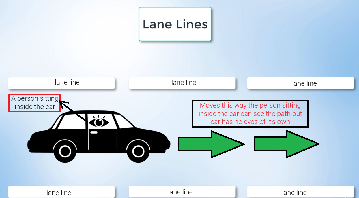
When we applied the computer vision algorithm to an image or video, the car was able to detect the lane lines itself using cameras or other sensors.

finding the lane lines in the series of camera images or camera frames.

Finding and identifying lane lines is our task:

Here, we have an image of lane lines below:

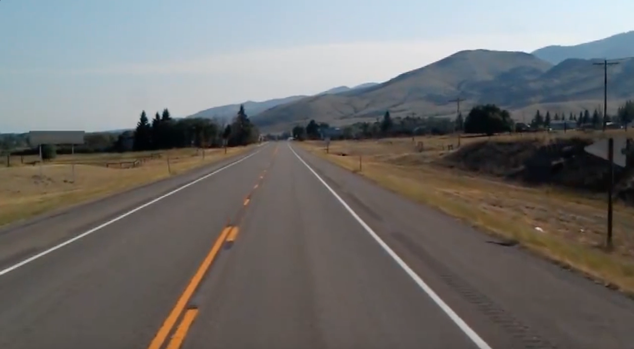
We can easily see the lane lines, but our goal is to make them detectable to the cameras, so our algorithm can identify them.

Step 1: Create a directory/folder name self_driving_car and inside it a folder named computer-vision and inside it another directory named finding-lanes then create a Python file named lanes.py and try to show this above image using the cv library. let's do this first step.

mkdir self_driving_car
cd self_driving_car

mkdir computer-vision
cd computer-vision

mkdir finding-lanes
cd finding-lanes
code .

When you are inside the finding-lanes folder creates a Python file named lanes.py and a folder named images and save the above lane image file.

In lanes.py file using two OpenCV methods imread() and imshow() methods we can able to read and show the images.

import cv2
image = cv2.imread('./images/test_image.jpg')
cv2.imshow('result', image)
cv2.waitKey(0)

• Importing the OpenCV library

import cv2

This line imports the OpenCV library in Python, which is widely used for computer vision and image-processing tasks.

• Reading an image

image = cv2.imread('./images/test_image.jpg')

Here, the cv2.imread() function is used to read an image file named "test_image.jpg" located in the "./images" directory relative to the current location of the script. The function reads the image and stores it in the variable named image.

• Displaying the image

cv2.imshow('result', image)

The cv2.imshow() function is used to display the image read in the previous step. The first argument is a string title for the window, and the second argument is the image variable, which contains the image data.

• Wait for User Input

cv2.waitKey(0)

This line of code waits indefinitely for a keyboard event. The argument passed to cv2.waitKey() specify the time (in milliseconds) the window should wait for a keyboard event. In this case, 0 signifies that the window will wait indefinitely until any key is pressed.

Step 2: Applying the canny edge detection technique

The goal of edge detection is to identify the boundaries of objects within images. in essence, we'll be using detection to try and find regions in an image where there is a sharp change in intensity (or) a sharp color change.

Edge Detection: Identifying sharp changes in intensity in adjacent pixels.

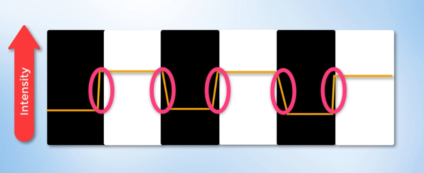
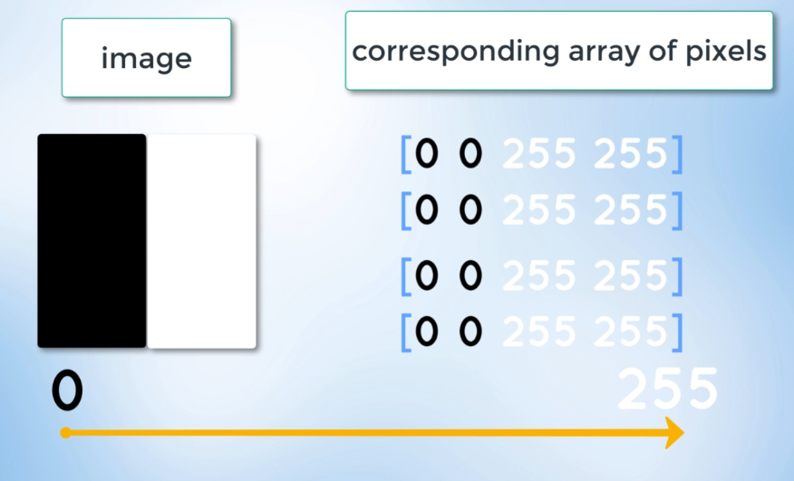
An image can mirror it as a matrix, an array of pixels, a pixel contains the light intensity at some location in the image. each pixel intensity is denoted by a numeric value that ranges from 0 to 255 and an intensity value of zero indicates no intensity.

It is completely black where values are 255 represent maximum intensity, and completely white where values are 0.

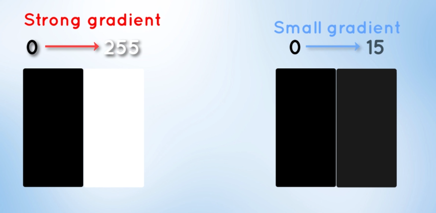
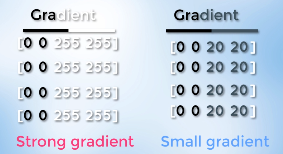
Here comes the gradient, which is the change in brightness over a series of pixels.

Gradient: Measure of change in brightness over adjacent pixels.

A strong gradient indicates a steep change whereas, a small gradient represents a shallow change.

Let's understand this concept using an example of a soccer ball. Below is the image given.

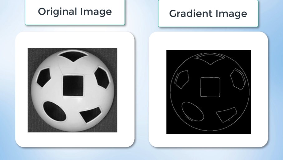
On the right-hand side of the image, you can see the gradient of the soccer ball. The white pixels indicate a sudden change in brightness which occurs at the points of the strengthened gradient. These bright pixels help us identify edges in our image.

An edge is defined by the difference in intensity values in adjacent pixels. Whenever there is a sharp change in intensity or a rapid change in brightness, we observe a strong gradient and a corresponding bright pixel in the gradient image. By tracing out all of these bright pixels, we can obtain the edges of the image.

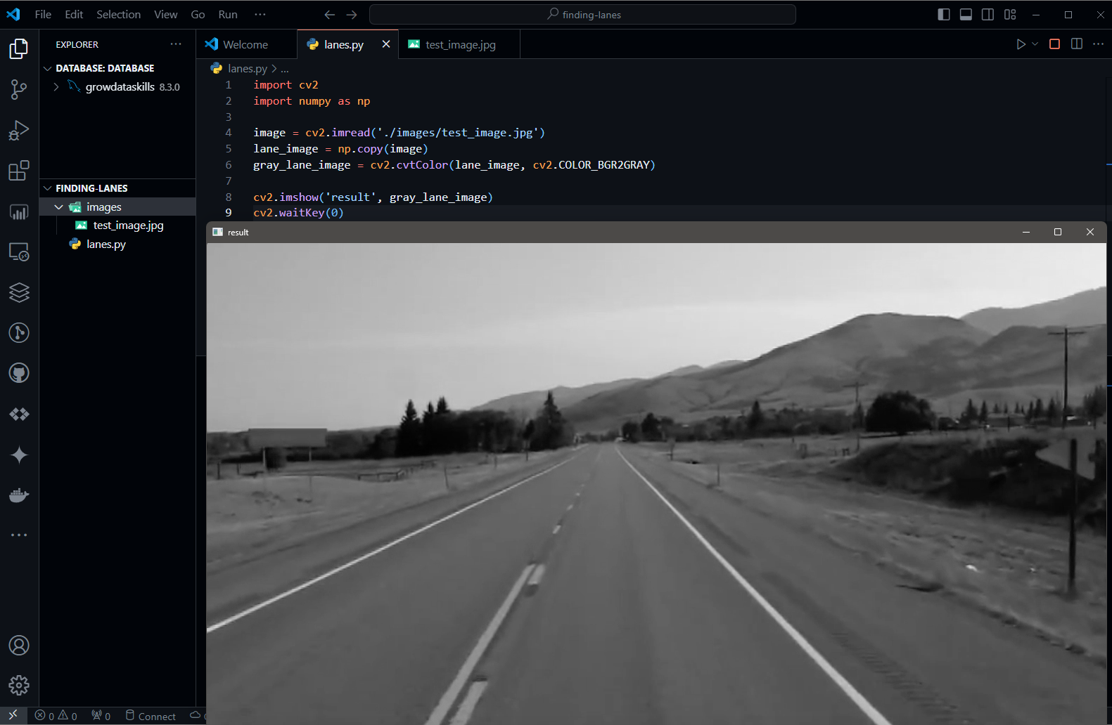
• Convert the lane image into grayscale: images are made up of pixels, A three-channel color image would have Red, Green, and Blue channels hence each pixel is a combination of three intensities values whereas, a grayscale image only has one channel for each pixel with one intensity value or one channel ranging from 0 to 255.

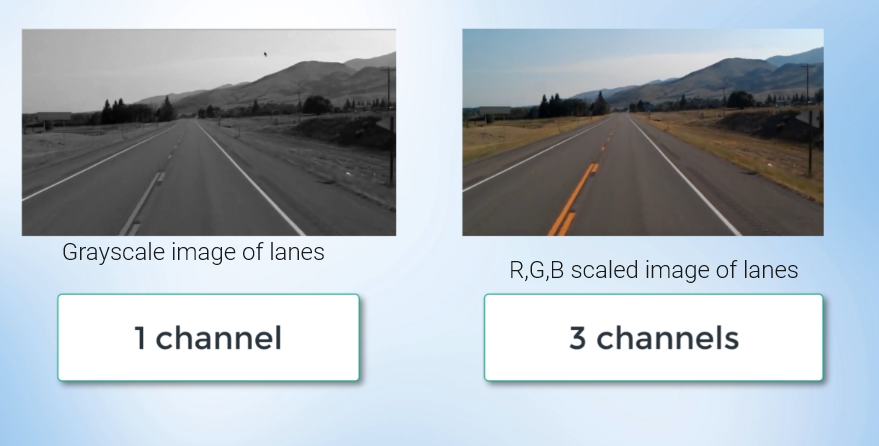
The point is that using grayscale image processing with a single channel is faster and less computationally intensive than processing a three-channel color image.

import cv2
import numpy as np

image = cv2.imread('./images/test_image.jpg')
lane_image = np.copy(image)
gray_lane_image = cv2.cvtColor(lane_image, cv2.COLOR_BGR2GRAY)

cv2.imshow('result', gray_lane_image)
cv2.waitKey(0)

• cv2.imread() reads the image file "test_image.jpg" from the specified path and stores it in the variable image.

• np.copy() is used to create a new copy of the image stored in the variable image. This ensures that any modifications made to the lane_image variable do not affect the original image.

• cv2.cvtColor() converts the color image stored, lane_image into a grayscale image. The function takes two arguments: the source image and the conversion code, cv2.COLOR_BGR2GRAY, which specifies the color space conversion.

• cv2.imshow() displays the grayscale image. The first argument is a string title for the window, and the second argument is the grayscale image variable, gray_lane_image.

• cv2.waitKey(0) waits indefinitely for a keyboard event. The argument 0 specifies the time (in milliseconds) the window should wait for a keyboard event. Here, it waits indefinitely until any key is pressed.

  Converting the Image to Grayscale and Displaying

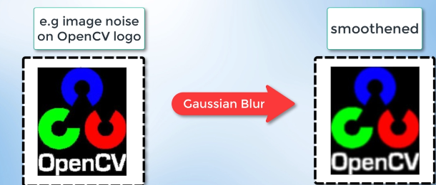
• Reducing noise and smoothening our image by applying Gaussian blur: When detecting edges we must filter out any image noise because image noise can create false edges and ultimately affect edge detection that's why it is imperative to filter it out and thus, smoothen the image.

Filtering out image noise and smoothening will be done with a Gaussian filter. The image is a collection of discrete pixels. Each of the pixels for a grayscale image is represented by a single number that describes the brightness of the pixel.

To smoothen the image, we have to modify the value of a pixel with the average of the pixel intensity around it. Averaging out the pixels in the image to reduce noise will be done with the kernel.

Essentially, this kernel of normally distributed numbers runs across our entire image and sets each pixel value to about the weighted average of its neighboring pixels, smoothing out the image.

import cv2
import numpy as np

image = cv2.imread('./images/test_image.jpg')
lane_image = np.copy(image)
gray = cv2.cvtColor(lane_image, cv2.COLOR_BGR2GRAY)
# Added to smoothening and reducing noise in image
blur = cv2.GaussianBlur(gray, (5, 5), 0)

cv2.imshow('With Gaussian blur', blur)
cv2.waitKey(0)

step 3: Applying Gaussian Blur

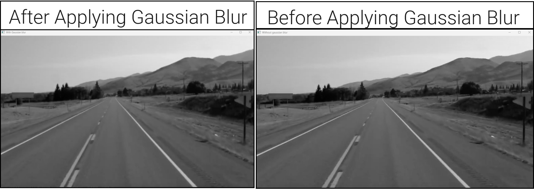
The cv2.GaussianBlur() function is used to apply Gaussian blur to the grayscale image. This is achieved to reduce noise and smoothen the image, which can be beneficial for subsequent image-processing tasks

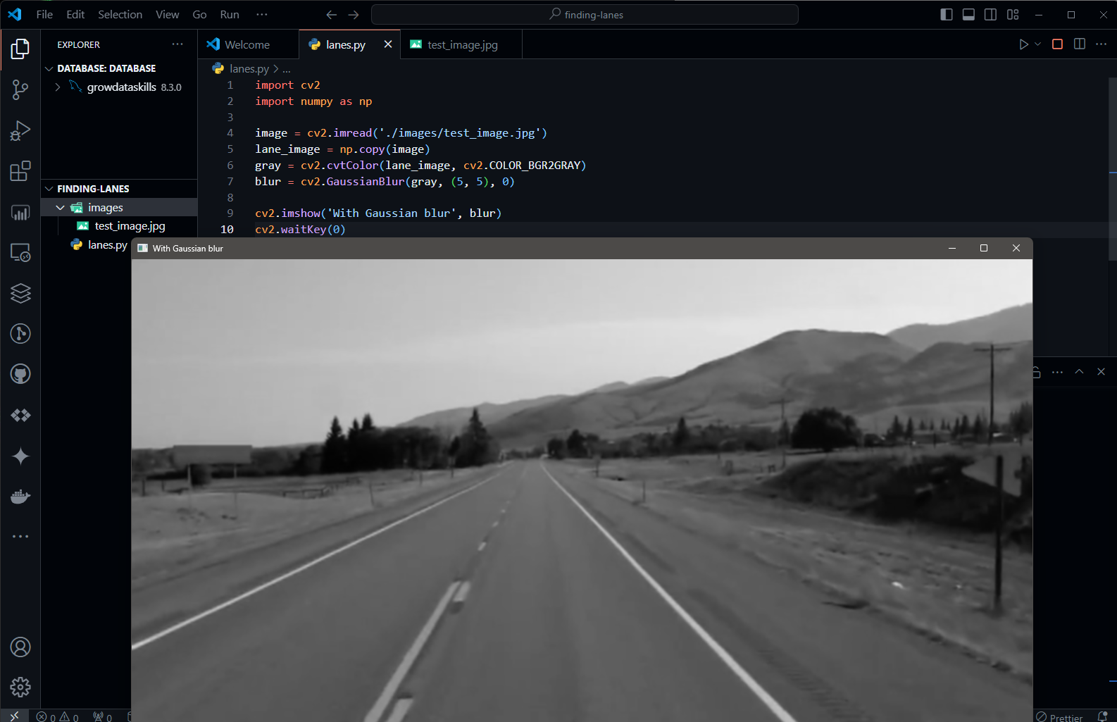
So let's see both images before applying Gaussian blur and with Gaussian blur:

• Applying the Canny Edge detection method: It helps to find edges in our image, an edge corresponds to a region in an image where there is a sharp change in intensity (or) a sharp change in color between adjacent pixels in the image. The change in brightness over a series of pixels is the gradient. Strong gradient. A strong gradient indicates a steep change whereas a small gradient indicates a shallow change.

  

  Images consist of pixels and can be interpreted as a matrix or an array of pixel intensities for calculating gradients in an image. Additionally, the image can be represented in a 2D coordinate space (X, Y), where the x-axis traverses the image and the y-axis corresponds to the image height, representing the number of columns and rows in the image. This means that the product of the width and height gives the total number of pixels in the image.

  

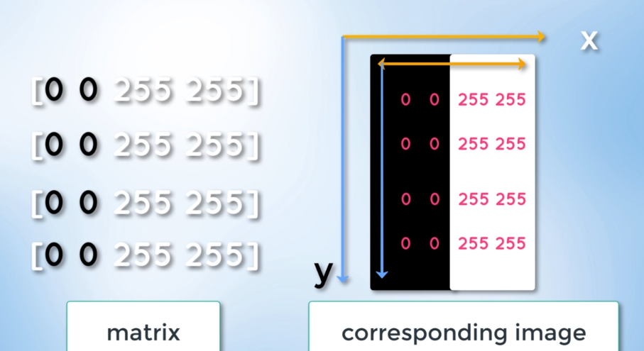
  The point is that we can view our image not only as an array but also as a continuous function of x and y. Being a mathematical function allows us to conduct mathematical operations.

  

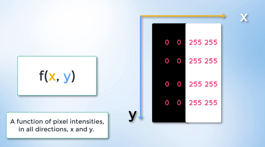
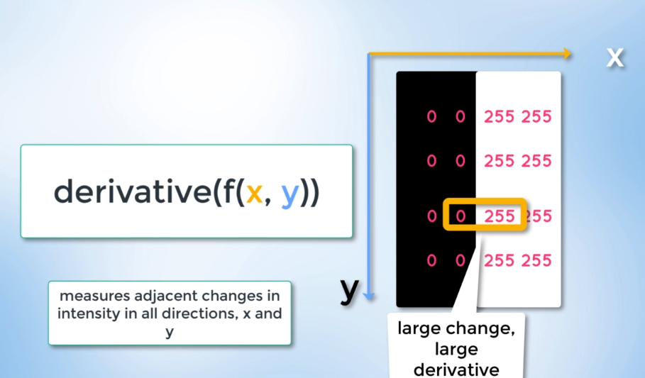
  So, which operator can we use to detect a quick change in the brightness of our image? The canny function calculates the derivative of our function in both the x and y directions, measuring the intensity change compared to neighboring pixels. A small derivative indicates a minor/small intensity change

  

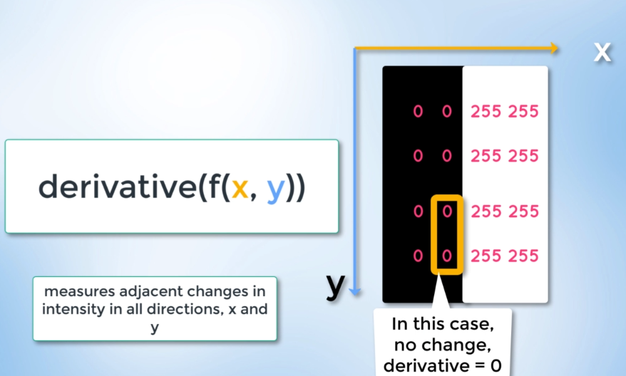
  while a large derivative indicates a big/significant change.

  

  When we call the canny function it does all of that for us.

• Canny Function: It computes the gradient in all directions of our blurred image and then traces our strongest gradients as a series of white pixels.

  

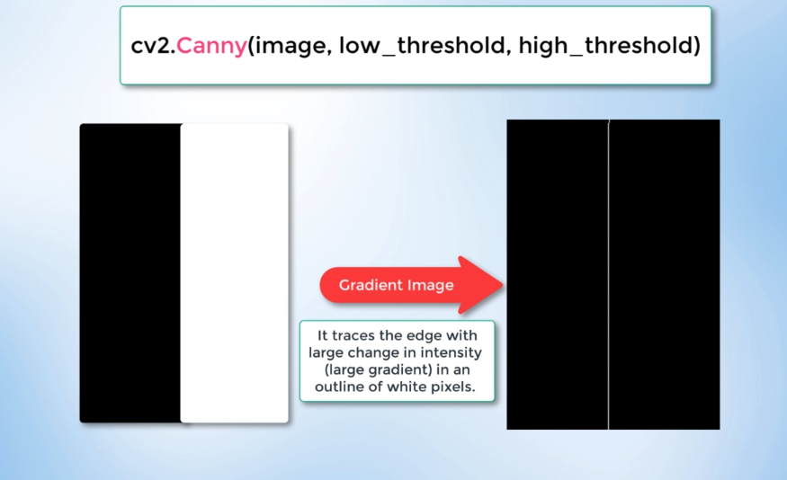
    cv2.Canny(image, low_threshold, high_threshold)
  

  low_threshold and high_threshold are used to isolate adjacent pixels based on gradient strength.

  

  If the gradient is higher than, high_thresholdit is considered an edge pixel; if it is below, low_threshold it is rejected. If the gradient is between both thresholds then it will be accepted only, if it is connected to a strong edge. The documentation itself, recommends using a ratio of 1:2 (or) 1:3 (or 50:150).

    import cv2
    import numpy as np
  
    image = cv2.imread('./images/test_image.jpg')
    lane_image = np.copy(image)
    gray  = cv2.cvtColor(lane_image, cv2.COLOR_BGR2GRAY)
    blur  = cv2.GaussianBlur(gray, (5, 5), 0)
    canny = cv2.Canny(blur, 50, 150)
  
    cv2.imshow('Image after applying canny function', canny)
    cv2.waitKey(0)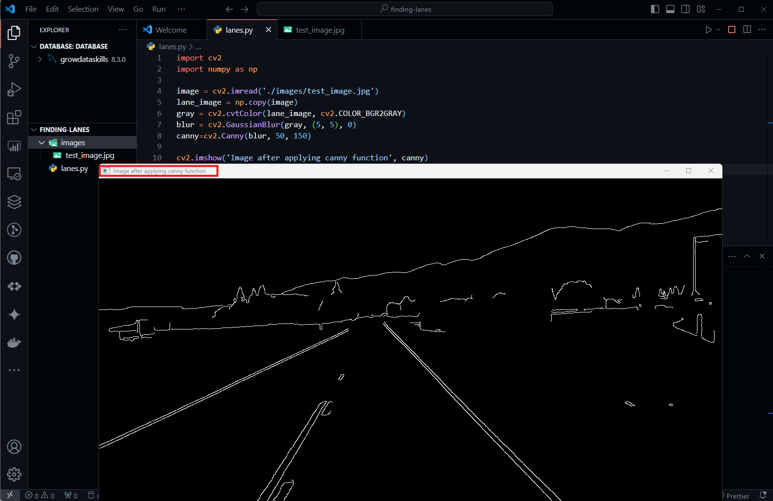
  

  

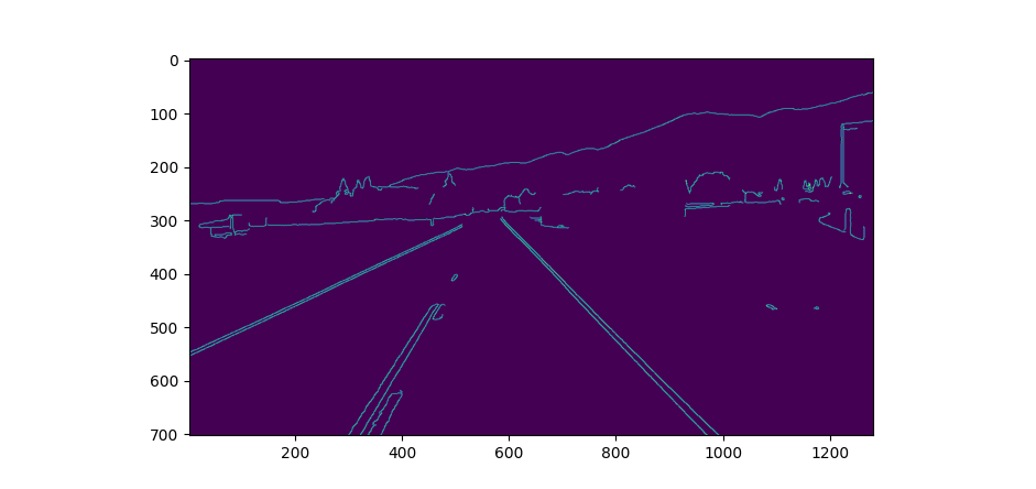
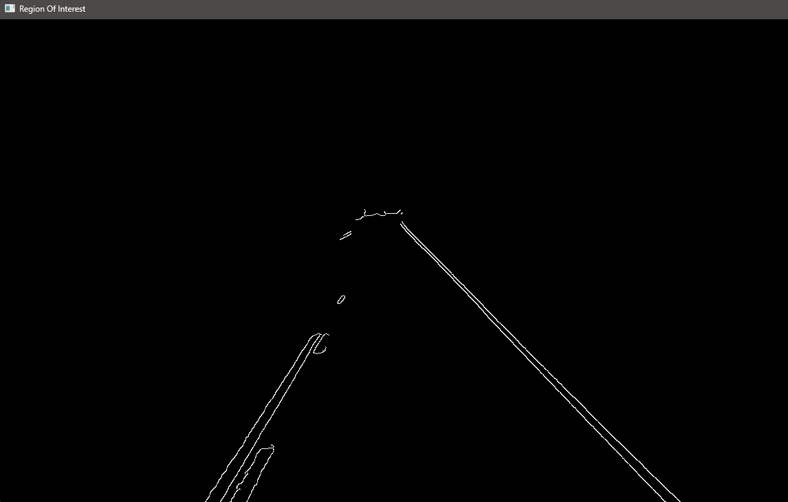
  Here is the gradient image which clearly outlines the edges corresponding to the sharpest changes in intensity gradients. Pixels exceeding the high_threshold are traced as bright, identifying adjacent pixels with the most rapid changes in brightness. Small changes below the low_threshold remain untraced and appear black.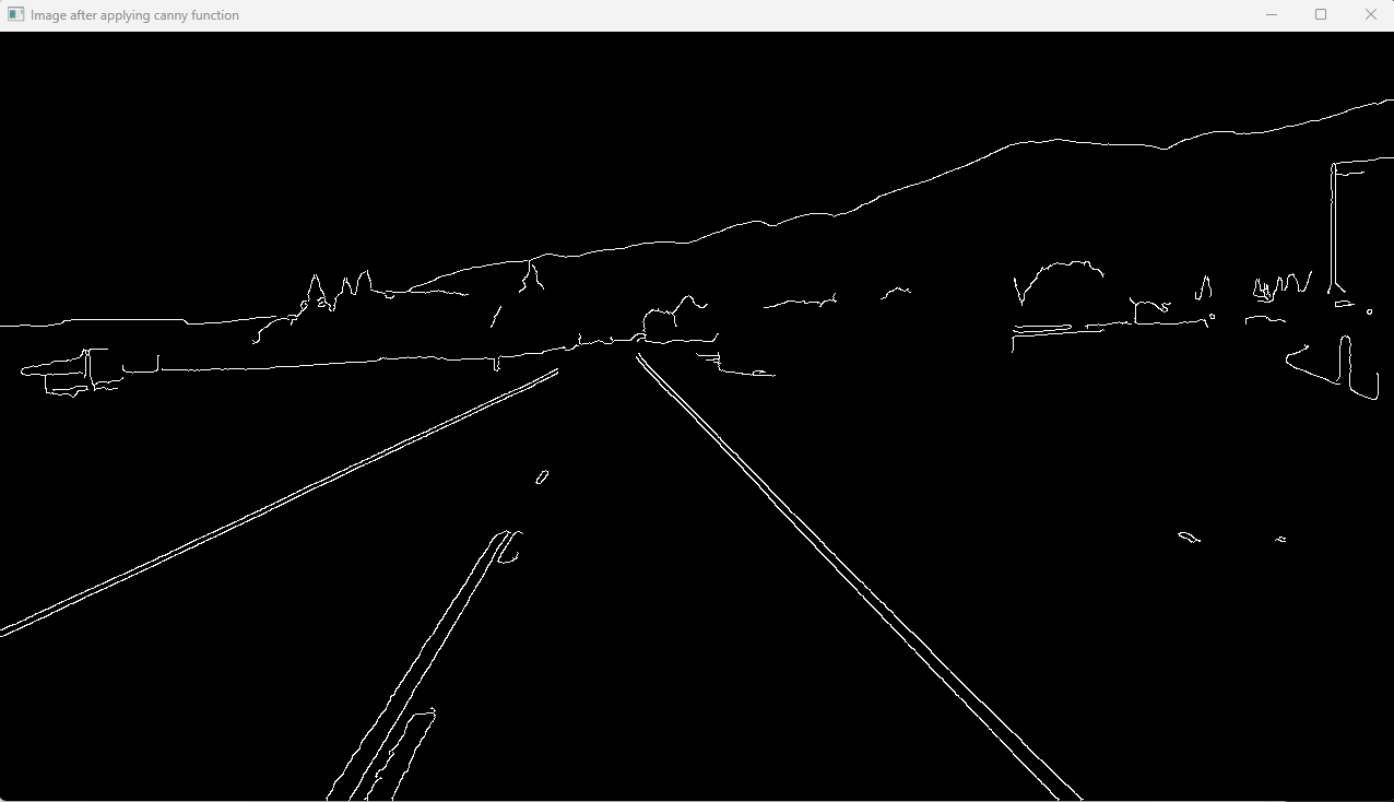

  

  Step 4: Find the region of interest and bitwise_and() to the image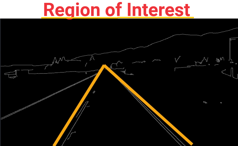

  

  let's structure the code in a modular format and show the image using Matplotlib.

•     import cv2
      import numpy as np
      import matplotlib.pyplot as plt
  
      # user define function to perform grayscaling, noise reduction and canny 
      # in one function
      def canny(image):
          gray  = cv2.cvtColor(lane_image, cv2.COLOR_BGR2GRAY)
          blur  = cv2.GaussianBlur(gray, (5, 5), 0)
          canny = cv2.Canny(blur, 50, 150)
          return canny
  
      image = cv2.imread('./images/test_image.jpg')
      lane_image = np.copy(image)
      canny = canny(lane_image)
  
      plt.imshow(canny) # instead of cv2 using plt 
      plt.show()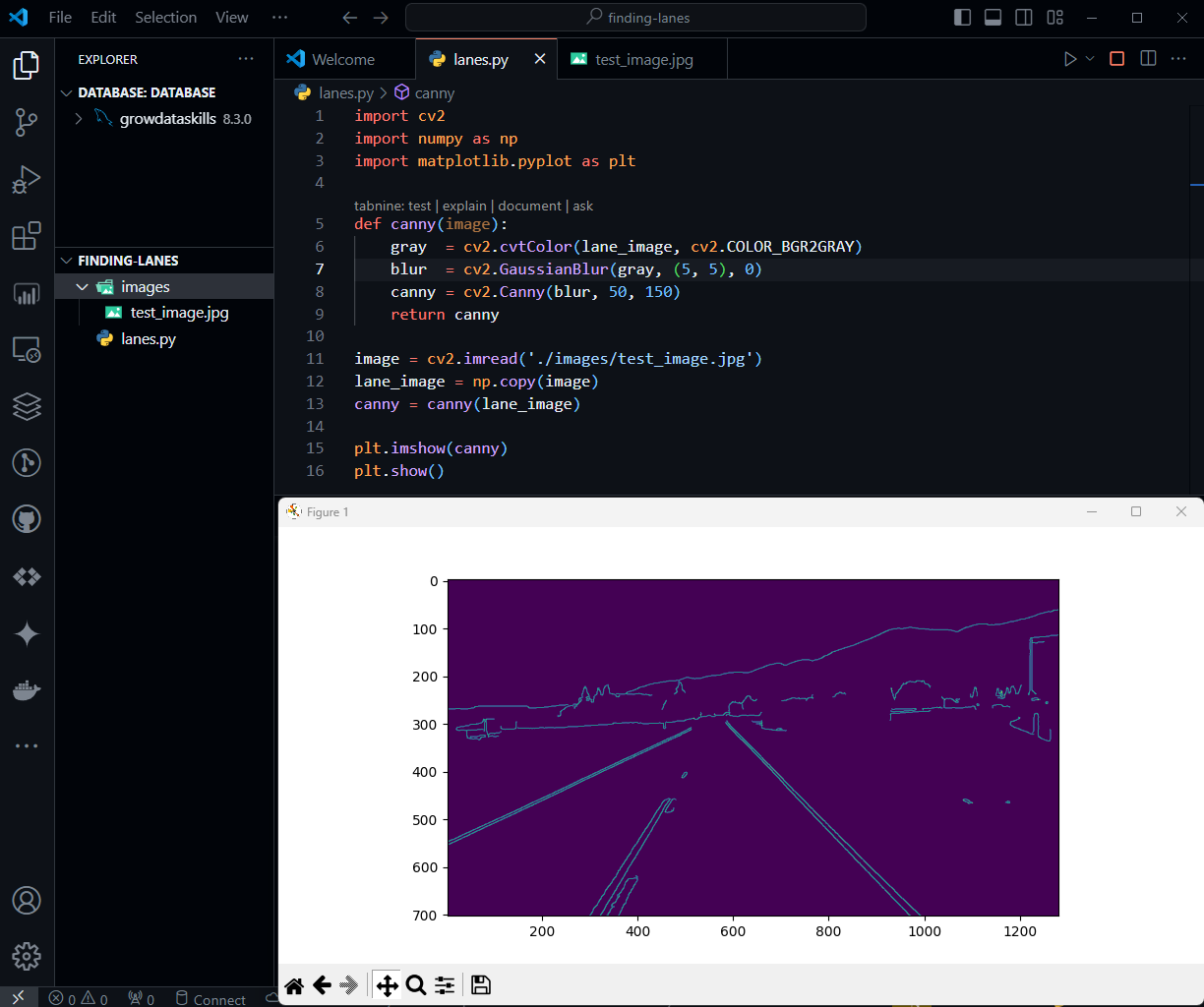
  

  

  

import cv2
import numpy as np
import matplotlib.pyplot as plt

def canny(image):
    gray  = cv2.cvtColor(lane_image, cv2.COLOR_BGR2GRAY)
    blur  = cv2.GaussianBlur(gray, (5, 5), 0)
    canny = cv2.Canny(blur, 50, 150)
    return canny

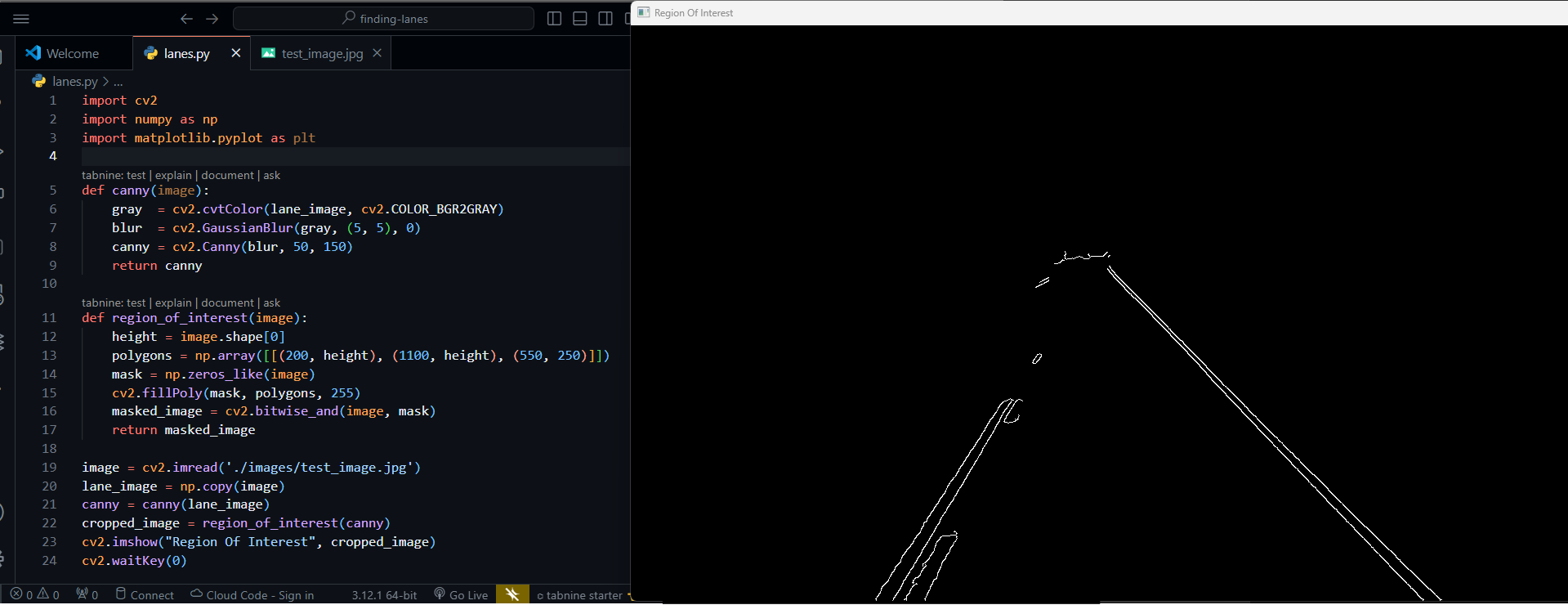
def region_of_interest(image):
    height = image.shape[0]
    polygons = np.array([[(200, height), (1100, height), (550, 250)]])
    mask = np.zeros_like(image)
    cv2.fillPoly(mask, polygons, 255)
    return mask

image = cv2.imread('./images/test_image.jpg')
lane_image = np.copy(image)
canny = canny(lane_image)

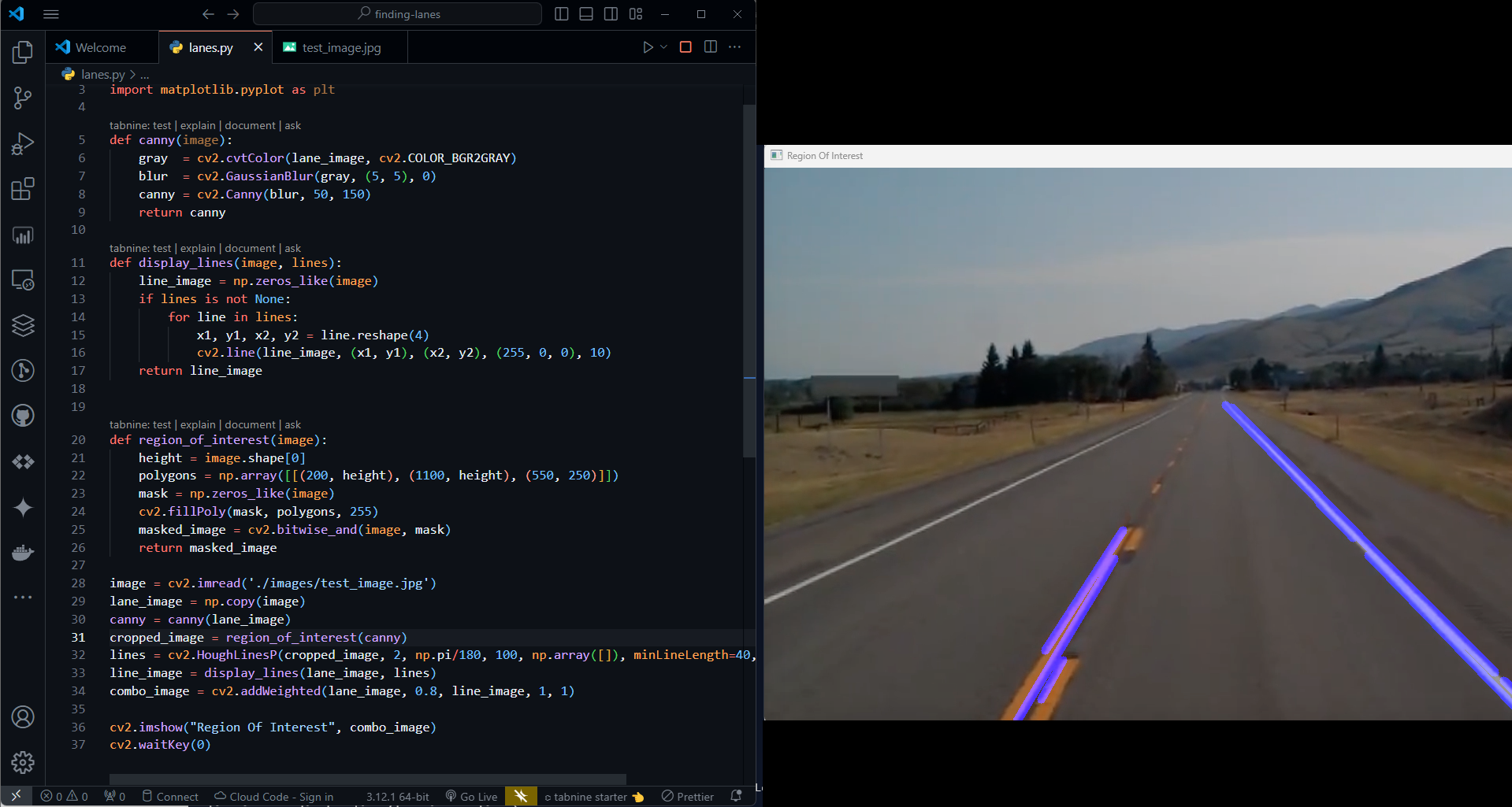
cv2.imshow("Region Of Interest", region_of_interest(canny))
cv2.waitKey(0)

Importing Libraries

import cv2
import numpy as np
import matplotlib.pyplot as plt

The code imports the necessary libraries, including cv2 for computer vision operations, numpy for array manipulation, and matplotlib.pyplot for plotting images.

1. Canny Edge Detection Function

    def canny(image):
        gray  = cv2.cvtColor(lane_image, cv2.COLOR_BGR2GRAY)
        blur  = cv2.GaussianBlur(gray, (5, 5), 0)
        canny = cv2.Canny(blur, 50, 150)
        return canny
   

   The canny() function is defined to take an input image and perform the following operations:

   • Convert the input image to grayscale using cv2.cvtColor().

   • Apply Gaussian blur to the grayscale image using cv2.GaussianBlur().

   • Perform Canny edge detection on the blurred image using cv2.Canny().

   • Return the resulting Canny edges.

2. Region of Interest Function

    def region_of_interest(image):
        height = image.shape[0]
        polygons = np.array([[(200, height), (1100, height), (550, 250)]])
        mask = np.zeros_like(image)
        cv2.fillPoly(mask, polygons, 255)
        return mask
   

   • The region_of_interest() function defines a region of interest on the input image and creates a mask.

   • It calculates the height of the input image, defines a polygon to represent the region of interest, creates a mask of zeros with the same dimensions as the input image, fills the defined polygon with white (255), and returns the resulting mask.

3. Image Processing

    image = cv2.imread('./images/test_image.jpg')
    lane_image = np.copy(image)
    canny = canny(lane_image)
   

   • The code reads an image from the file "test_image.jpg" and stores it in the variable image. The function cv2.imread() is used for this purpose.

   • The np.copy() function is used to create a copy of the original image, stored in the variable lane_image.

   • The canny() function is then called with lane_image as the input, and the resulting Canny edges are stored in the variable canny.

4. Displaying the Masked Image

    cv2.imshow("Region Of Interest", region_of_interest(canny))
    cv2.waitKey(0)
   

   • The region_of_interest() function is called with the Canny edges as input to create a masked image.

   • The masked image is displayed in a window titled "Region Of Interest" using cv2.imshow().

   • The cv2.waitKey(0) statement waits indefinitely for a keyboard event, allowing the user to view the displayed image until a key is pressed.

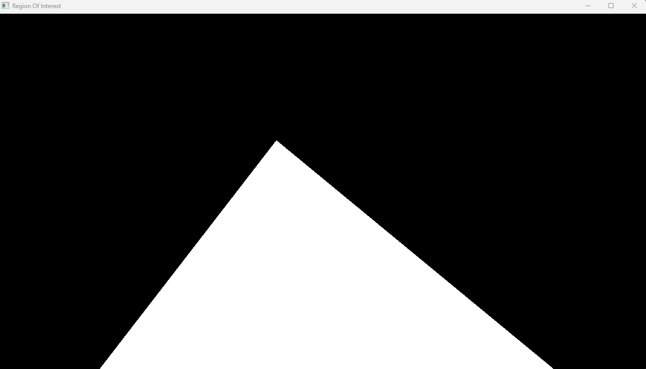
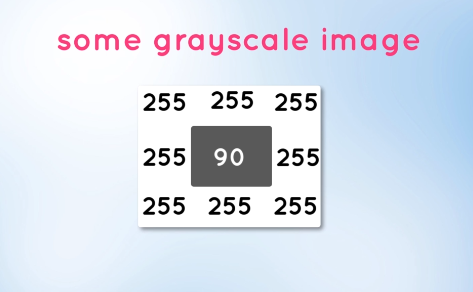
let's take the pixel representation of this resized image.

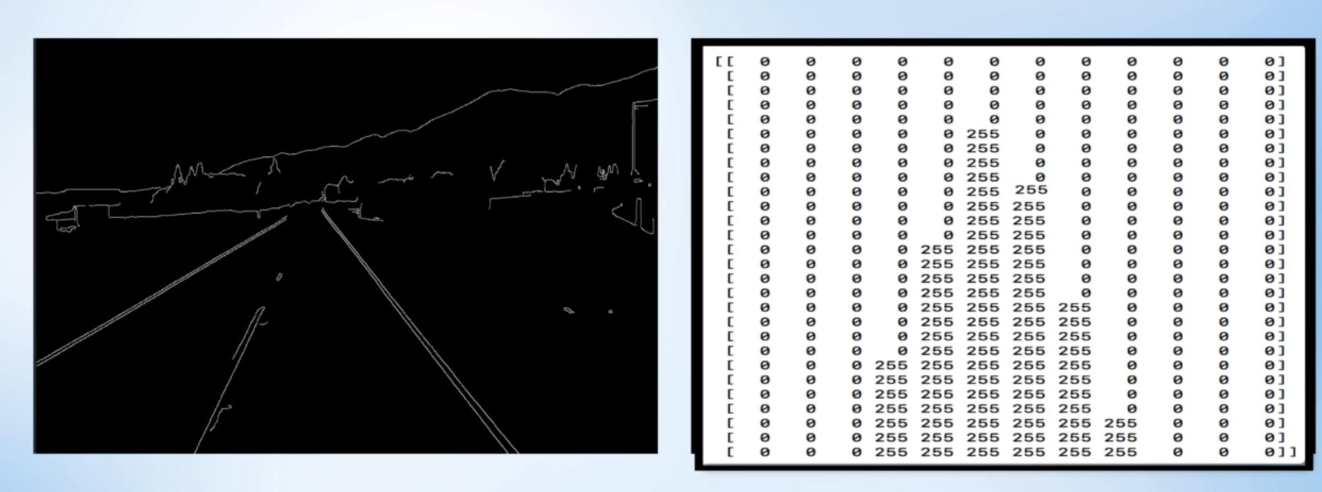
A triangular polygon translates to pixel intensities of 255 as white and the block surrounding region translates to pixel intensities of zeroes.

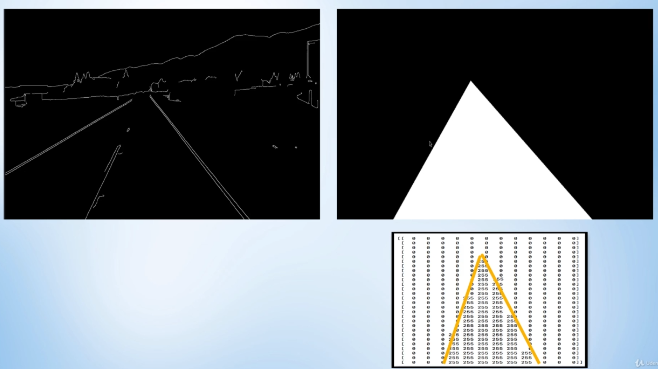
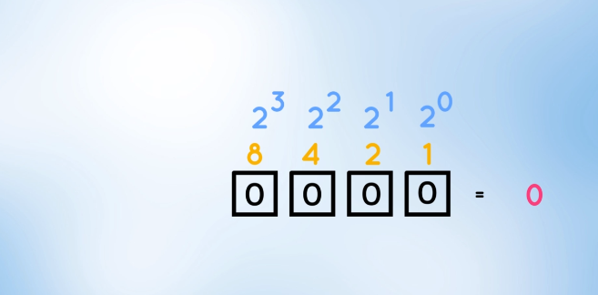
The binary representation of zero:

the binary representation of 255:

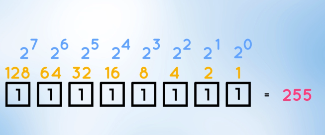
2⁷ + 2⁶ + 2⁵ + 2⁴ + 2³ + 2² + 2¹ + 2⁰ \= 255 [1, 1, 1, 1, 1, 1, 1, 1]. It is the maximum representable value by an 8-bit byte. So we conclude the surrounding region is completely black then, its binary representation is all zeroes [0, 0, 0, 0, 0, 0, 0, 0].

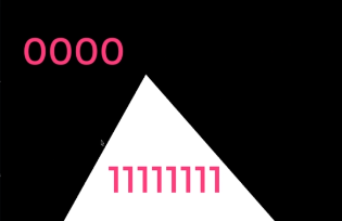
We can apply the bitwise AND operation between the two images. The bitwise AND operation occurs element-wise between the two arrays of pixels.

import cv2
import numpy as np
import matplotlib.pyplot as plt

def canny(image):
    gray  = cv2.cvtColor(lane_image, cv2.COLOR_BGR2GRAY)
    blur  = cv2.GaussianBlur(gray, (5, 5), 0)
    canny = cv2.Canny(blur, 50, 150)
    return canny

def region_of_interest(image):
    height = image.shape[0]
    polygons = np.array([[(200, height), (1100, height), (550, 250)]])
    mask = np.zeros_like(image)
    cv2.fillPoly(mask, polygons, 255)
    masked_image = cv2.bitwise_and(image, mask)
    return masked_image

image = cv2.imread('./images/test_image.jpg')
lane_image = np.copy(image)
canny = canny(lane_image)
cropped_image = region_of_interest(canny)
cv2.imshow("Region Of Interest", cropped_image)
cv2.waitKey(0)

Step 5: Applying Hough transform

The Hough transform is a technique used in image processing and computer vision to detect shapes, particularly lines and curves, within an image. Here's a simple explanation of the Hough transform:

1. Basic Concept: Imagine you have an image with a bunch of edge pixels that form a line. The Hough transform helps you find which straight line those edge pixels belong to.

    import cv2
   
    # Creating an image with a line
    image = np.zeros((200, 200), dtype=np.uint8)
    cv2.line(image, (50, 50), (150, 150), 255, 1)
   
    cv2.imshow("Image with Line", image)
    cv2.waitKey(0)
    cv2.destroyAllWindows()
   

2. Parameter Space: The Hough transform works by representing lines in a different space called the "Hough space" or "parameter space." Instead of the usual x-y coordinates of a line, Hough space uses parameters like slope (m) and intercept (c) for a normal line equation (y = mx + c).

    import numpy as np
   
    # Regular line equation: y = mx + c
    # Hough space: m - Slope, c - Intercept
    # Image to Hough Transform space conversion
    m = np.arange(-10, 10, 1)
    c = np.arange(0, 200, 1)
   
    # Visualizing Hough space
    M, C = np.meshgrid(m, c)
   
    print("Hough Space: ")
    print("Slope (m):", M)
    print("Intercept (c):", C)
   

3. Voting Process:

   • For each edge point in the image, the Hough transform "votes" for all possible lines that could pass through it in the Hough space.

   • Each edge point contributes to a curve in the Hough space, and the intersection of these curves indicates the parameters of the line that fits the edge points.

    # Imaginary edge points
    edge_points = [(80, 75), (90, 85), (100, 95)]

    for point in edge_points:
        m = (point[1] - 50) / (point[0] - 50)  # Calculate slope
        c = point[1] - m * point[0]  # Calculate intercept
        print("Voting for line with slope m =", m, "and intercept c =", c)

4. Accumulator Array: This "voting" process is often visualized using an "accumulator array," which is a grid in the Hough space. Each cell in the grid accumulates votes for a particular line defined by its parameters.

# Setting up accumulator array
accumulator = np.zeros((200, 200), dtype=np.uint8)

# Casting votes for the line: y = mx + c
for m, c in zip(m_vals, c_vals):
    y = np.round(m * x + c).astype(int)
    accumulator[y, x] += 1

Finding Peaks:

After all edge points have been voted, peaks in the accumulator array indicate the most likely parameters of the lines in the image.

These peaks correspond to the parameters of the lines that were "popular" among the edge points.

# Find peaks in the accumulator array
peaks = cv2.HoughLines(accumulator, 1, np.pi / 180, threshold=50)

# Plotting the detected lines in the original image
for peak in peaks:
    rho, theta = peak[0]
    a = np.cos(theta)
    b = np.sin(theta)
    x0 = a * rho
    y0 = b * rho
    x1 = int(x0 + 1000 * (-b))
    y1 = int(y0 + 1000 * (a))
    x2 = int(x0 - 1000 * (-b))
    y2 = int(y0 - 1000 * (a)
    cv2.line(image, (x1, y1), (x2, y2), (0, 255, 0), 2)

import cv2
import numpy as np
import matplotlib.pyplot as plt

def canny(image):
    gray  = cv2.cvtColor(lane_image, cv2.COLOR_BGR2GRAY)
    blur  = cv2.GaussianBlur(gray, (5, 5), 0)
    canny = cv2.Canny(blur, 50, 150)
    return canny

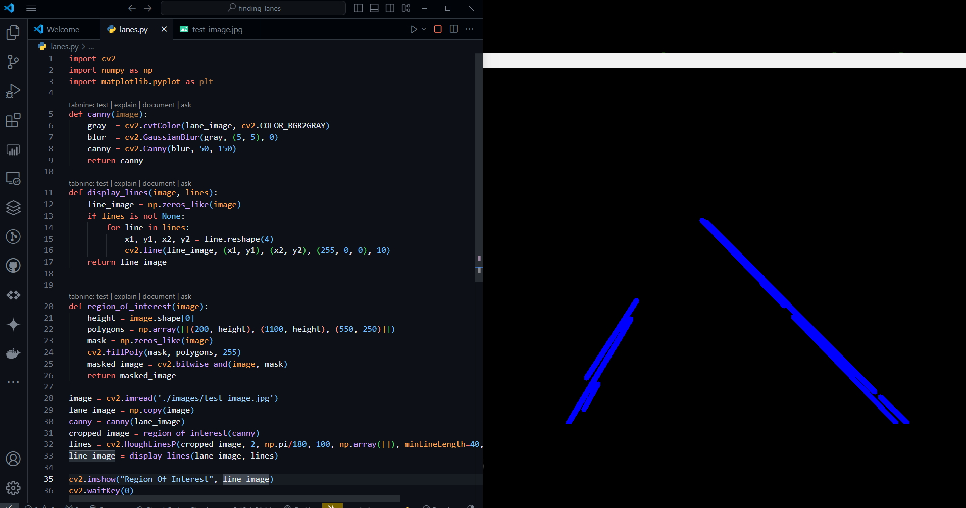
def display_lines(image, lines):
    line_image = np.zeros_like(image)
    if lines is not None:
        for line in lines:
            x1, y1, x2, y2 = line.reshape(4)
            cv2.line(line_image, (x1, y1), (x2, y2), (255, 0, 0), 10)
    return line_image


def region_of_interest(image):
    height = image.shape[0]
    polygons = np.array([[(200, height), (1100, height), (550, 250)]])
    mask = np.zeros_like(image)
    cv2.fillPoly(mask, polygons, 255)
    masked_image = cv2.bitwise_and(image, mask)
    return masked_image

image = cv2.imread('./images/test_image.jpg')
lane_image = np.copy(image)
canny = canny(lane_image)
cropped_image = region_of_interest(canny)
lines = cv2.HoughLinesP(cropped_image, 2, np.pi/180, 100, np.array([]), minLineLength=40, maxLineGap=5)
line_image = display_lines(lane_image, lines)

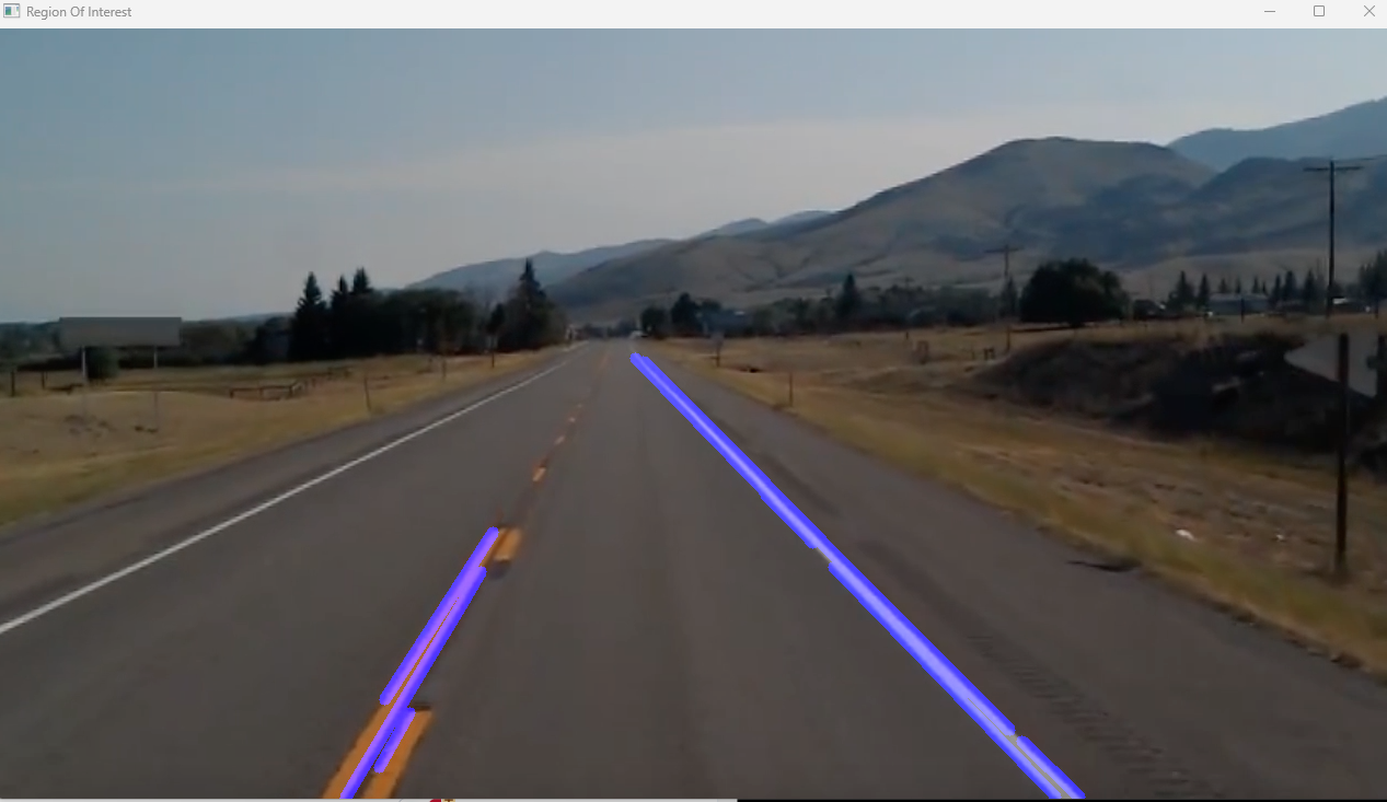
cv2.imshow("Region Of Interest", line_image)
cv2.waitKey(0)

• The display_lines() function takes the original image and detected lines as input.

• It creates a blank image of the same size as the input image and draws the detected lines on it using cv2.line().

• The function then returns the image with the detected lines drawn on it.

• The Hough line transform is applied to the cropped image cv2.HoughLinesP() to detect the lines. Then, the detected lines are drawn on a separate image display_lines() and stored in line_image.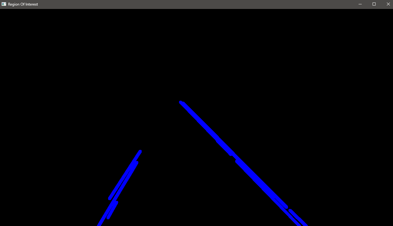

  

  ```python import cv2 import numpy as np import matplotlib.pyplot as plt

  def canny(image): gray = cv2.cvtColor(lane_image, cv2.COLOR_BGR2GRAY) blur = cv2.GaussianBlur(gray, (5, 5), 0) canny = cv2.Canny(blur, 50, 150) return canny

  def display_lines(image, lines): line_image = np.zeros_like(image) if lines is not None: for line in lines: x1, y1, x2, y2 = line.reshape(4) cv2.line(line_image, (x1, y1), (x2, y2), (255, 0, 0), 10) return line_image

def region_of_interest(image): height = image.shape[0] polygons = np.array([[(200, height), (1100, height), (550, 250)]]) mask = np.zeros_like(image) cv2.fillPoly(mask, polygons, 255) masked_image = cv2.bitwise_and(image, mask) return masked_image

image = cv2.imread('./images/test_image.jpg') lane_image = np.copy(image) canny = canny(lane_image) cropped_image = region_of_interest(canny) lines = cv2.HoughLinesP(cropped_image, 2, np.pi/180, 100, np.array([]), minLineLength=40, maxLineGap=5) line_image = display_lines(lane_image, lines) combo_image = cv2.addWeighted(lane_image, 0.8, line_image, 1, 1)

cv2.imshow("Region Of Interest", combo_image) cv2.waitKey(0)

    * Finally, the detected lines are combined with the original image using `cv2.addWeighted()` and stored in `combo_image`.

        ```python
        combo_image = cv2.addWeighted(lane_image, 0.8, line_image, 1, 1)

• Displaying the Result:

  

import cv2
import numpy as np

def make_coordinates(image, line_parameters):
    slope, intercept = line_parameters
    y1 = int(image.shape[0])
    y2 = int(y1*3/5)        
    x1 = int((y1 - intercept)/slope)
    x2 = int((y2 - intercept)/slope)
    return [[x1, y1, x2, y2]]

def average_slope_intercept(image, lines):
    left_fit    = []
    right_fit   = []
    if lines is None:
        return None
    for line in lines:
        for x1, y1, x2, y2 in line:
            parameters = np.polyfit((x1,x2), (y1,y2), 1)
            slope = parameters[0]
            intercept = parameters[1]
            if slope < 0: # y is reversed in image
                left_fit.append((slope, intercept))
            else:
                right_fit.append((slope, intercept))

    # add more weight to longer lines
    left_fit_average  = np.average(left_fit, axis=0)
    right_fit_average = np.average(right_fit, axis=0)
    left_line  = make_coordinates(image, left_fit_average)
    right_line = make_coordinates(image, right_fit_average)
    averaged_lines = [left_line, right_line]
    return averaged_lines

def canny(image):
    gray = cv2.cvtColor(image, cv2.COLOR_RGB2GRAY)
    blur = cv2.GaussianBlur(gray,(5, 5),0)
    canny = cv2.Canny(gray, 50, 150)
    return canny

def display_lines(image, lines):
    line_image = np.zeros_like(image)
    if lines is not None:
        for line in lines:
            for x1, y1, x2, y2 in line:
                cv2.line(line_image,(x1,y1),(x2,y2),(255,0,0),10)
    return line_image

def region_of_interest(image):
    height = image.shape[0]
    mask = np.zeros_like(image)
    polygons = np.array([[(200, height), (550, 250), (1100, height),]], np.int32)
    cv2.fillPoly(mask, polygons, 255)
    masked_image = cv2.bitwise_and(image, mask)
    return masked_image


image = cv2.imread('./images/test_image.jpg')
lane_image = np.copy(image)
lane_canny = canny(lane_image)
cropped_canny = region_of_interest(lane_canny)
lines = cv2.HoughLinesP(cropped_canny, 2, np.pi/180, 100, np.array([]), minLineLength=40,maxLineGap=5)
averaged_lines = average_slope_intercept(image, lines)
line_image = display_lines(lane_image, averaged_lines)
combo_image = cv2.addWeighted(lane_image, 0.8, line_image, 1, 1)

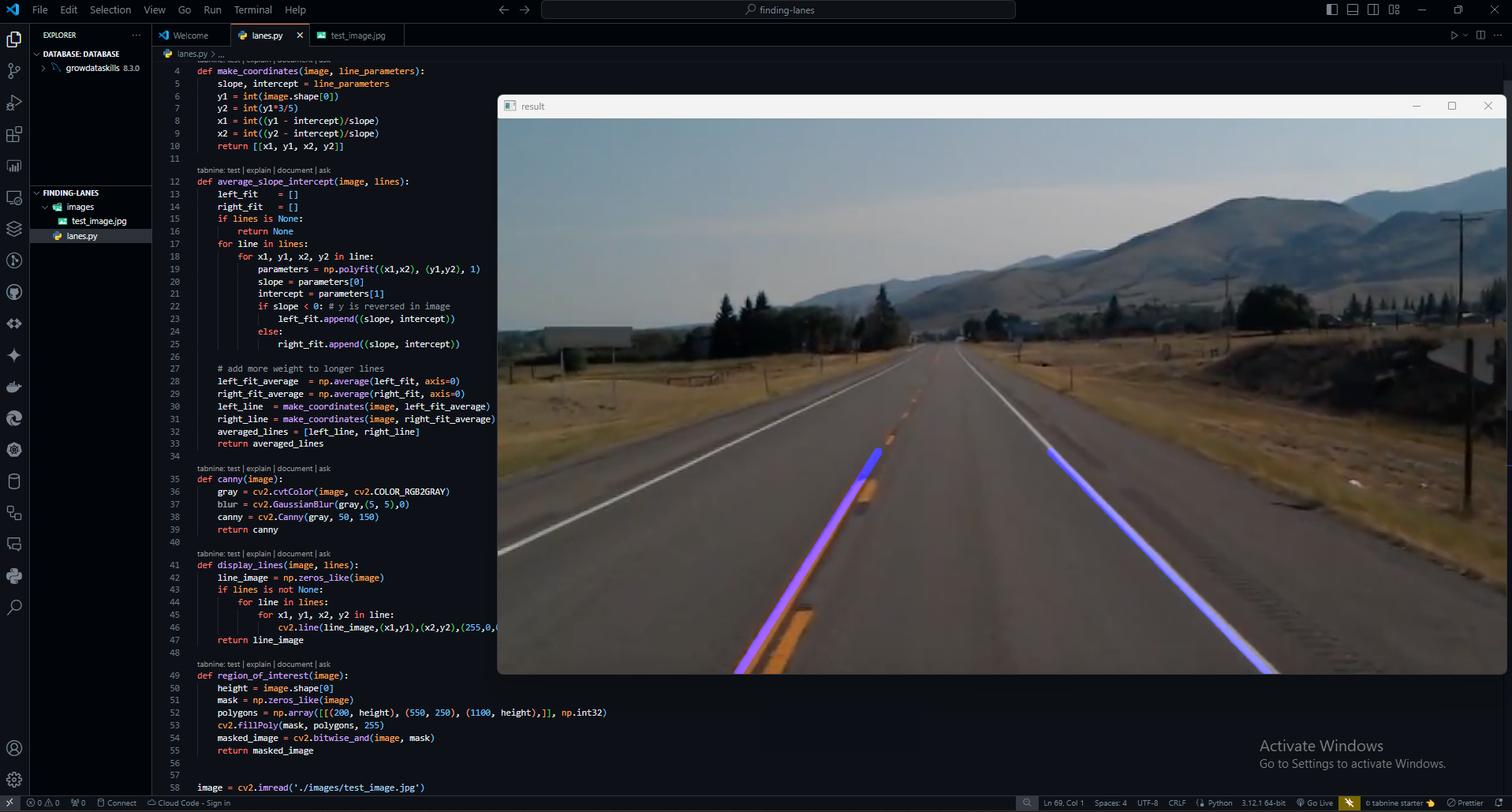
cv2.imshow("result", combo_image)
cv2.waitKey(0)

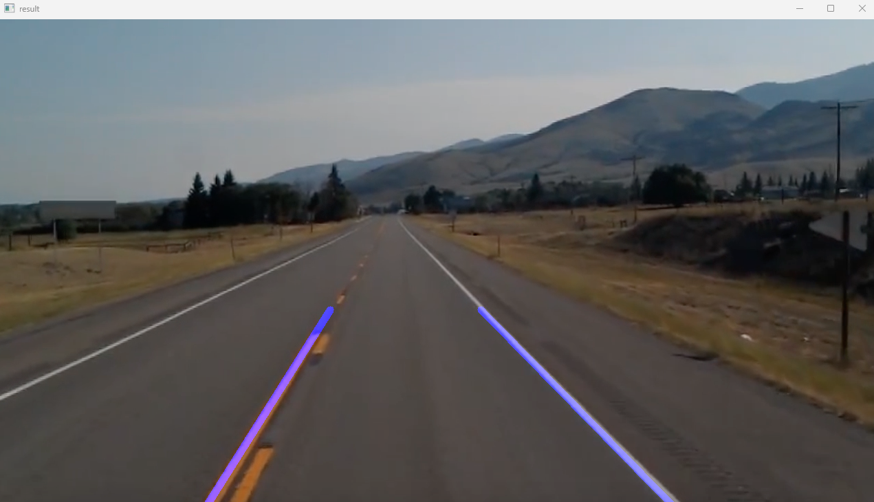
Defining Coordinates and Averaging Slope Intercept:

• The function make_coordinates() calculates the coordinates of the lanes based on the line parameters, and it returns a list of line coordinates.

• The function average_slope_intercept() takes the image and detected lines as input and performs the following operations:

  • Iterates through the detected lines and calculates their slopes and intercepts.

  • Groups the lines into left and right lanes based on their slopes (negative for the left lane and positive for the right lane).

  • Averages the slopes and intercepts of the left and right lanes, giving more weight to longer lines.

  • Calculates the coordinates of the averaged left and right lines using the make_coordinates() function and returns them as a list of averaged lines.

Canny Edge Detection: The canny() function performs Canny edge detection on the input image using the grayscale conversion, Gaussian blur, and the Canny edge detection algorithm. The resulting edges are returned.

Displaying Detected Lines: The display_lines() function takes the original image and the detected lines as input, and it draws the detected lines on a blank image.

Defining the Region of Interest: The region_of_interest() function defines a region of interest using a polygon and creates a mask for the input image. It then isolates the region of interest using the mask and returns the masked image.

Image Processing for Lane Detection:

• The code reads an image from the file "test_image.jpg" and stores it in the variable image. A copy of the original image is made and stored in lane_image.

• Canny edge detection is applied to lane_image, and the result is stored in lane_canny.

• The region of interest is isolated using region_of_interest(), and the resulting image is stored in cropped_canny.

• Hough line transform is applied to the cropped Canny image using cv2.HoughLinesP() to detect the lines. The detected lines are then averaged using the average_slope_intercept() function.

• The function display_lines() is used to draw the averaged lines on a blank image, and the result is stored in line_image.

• The original image and the detected lines are combined using cv2.addWeighted() and stored in combo_image.

Now, we applied it all in an image let's apply the same in a video.

import cv2
import numpy as np

def make_points(image, line):
    slope, intercept = line
    y1 = int(image.shape[0])
    y2 = int(y1*3/5)        
    x1 = int((y1 - intercept)/slope)
    x2 = int((y2 - intercept)/slope)
    return [[x1, y1, x2, y2]]

def average_slope_intercept(image, lines):
    left_fit    = []
    right_fit   = []
    if lines is None:
        return None
    for line in lines:
        for x1, y1, x2, y2 in line:
            fit = np.polyfit((x1,x2), (y1,y2), 1)
            slope = fit[0]
            intercept = fit[1]
            if slope < 0: # y is reversed in image
                left_fit.append((slope, intercept))
            else:
                right_fit.append((slope, intercept))
    # add more weight to longer lines
    left_fit_average  = np.average(left_fit, axis=0)
    right_fit_average = np.average(right_fit, axis=0)
    left_line  = make_points(image, left_fit_average)
    right_line = make_points(image, right_fit_average)
    averaged_lines = [left_line, right_line]
    return averaged_lines

def canny(img):
    gray = cv2.cvtColor(img, cv2.COLOR_RGB2GRAY)
    kernel = 5
    blur = cv2.GaussianBlur(gray,(kernel, kernel),0)
    canny = cv2.Canny(gray, 50, 150)
    return canny

def display_lines(img,lines):
    line_image = np.zeros_like(img)
    if lines is not None:
        for line in lines:
            for x1, y1, x2, y2 in line:
                cv2.line(line_image,(x1,y1),(x2,y2),(255,0,0),10)
    return line_image

def region_of_interest(canny):
    height = canny.shape[0]
    width = canny.shape[1]
    mask = np.zeros_like(canny)

    triangle = np.array([[
    (200, height),
    (550, 250),
    (1100, height),]], np.int32)

    cv2.fillPoly(mask, triangle, 255)
    masked_image = cv2.bitwise_and(canny, mask)
    return masked_image

cap = cv2.VideoCapture("./videos/test_video.mp4")
while(cap.isOpened()):
    _, frame = cap.read()
    canny_image = canny(frame)
    cropped_canny = region_of_interest(canny_image)
    lines = cv2.HoughLinesP(cropped_canny, 2, np.pi/180, 100, np.array([]), minLineLength=40,maxLineGap=5)
    averaged_lines = average_slope_intercept(frame, lines)
    line_image = display_lines(frame, averaged_lines)
    combo_image = cv2.addWeighted(frame, 0.8, line_image, 1, 1)
    cv2.imshow("result", combo_image)
    if cv2.waitKey(1) & 0xFF == ord('q'):
        break

cap.release()
cv2.destroyAllWindows()

Defining Helper Functions:

• The make_points() function takes an image and a line's slope and intercept parameters as input. It calculates the coordinates of the endpoints of the line based on the image shape and the line parameters and returns a list of line coordinates.

• The average_slope_intercept() function takes the image and detected lines as input and performs the following operations:

  • Iterates through the detected lines and calculates their slopes and intercepts using linear regression (polyfit).

  • Groups the lines into left and right lanes based on their slopes (negative for the left lane and positive for the right lane).

  • Averages the slopes and intercepts of the left and right lanes, giving more weight to longer lines, and calculates the coordinates of the averaged left and right lines using the make_points() function. It then returns a list of averaged lines.

• The canny(), the function performs Canny edge detection on the input image using the grayscale conversion, Gaussian blur, and Canny edge detection algorithm. The resulting edges are returned.

• The display_lines() function takes the original image and the detected lines as input, draws the detected lines on a blank image, and returns the resulting image.

• The region_of_interest() function defines a region of interest using a polygon, creates a mask for the input image, isolates the region of interest using the mask, and returns the masked image.

Processing Video Frames:

• The code takes video frames from the file "test_video.mp4" and processes each frame in a loop.

• For each frame, it performs the following operations:

  • Applies Canny edge detection to the frame using the canny() function.

  • Isolates the region of interest within the Canny image using the region_of_interest() function.

  • Uses the Hough line transform to detect lines in the cropped Canny image.

  • Averages and calculates the coordinates of the detected lines using the average_slope_intercept() function.

  • Draws the averaged lines on a blank image using the display_lines() function and combines the original frame with the detected lines using cv2.addWeighted().

  • Displays the resulting image with the detected and averaged lines in a window titled "result".

• The processing loop continues until the user presses the 'q' key, at which point the video stream is released and all windows are closed using cap.release() and cv2.destroyAllWindows().

cap = cv2.VideoCapture("./videos/test_video.mp4")
while(cap.isOpened()):
    _, frame = cap.read()
    canny_image = canny(frame)
    cropped_canny = region_of_interest(canny_image)
    lines = cv2.HoughLinesP(cropped_canny, 2, np.pi/180, 100, np.array([]), minLineLength=40,maxLineGap=5)
    averaged_lines = average_slope_intercept(frame, lines)
    line_image = display_lines(frame, averaged_lines)
    combo_image = cv2.addWeighted(frame, 0.8, line_image, 1, 1)
    cv2.imshow("result", combo_image)
    if cv2.waitKey(1) & 0xFF == ord('q'):
        break

cap.release()

# Explaination:
# Open the video file for reading frames
cap = cv2.VideoCapture("./videos/test_video.mp4")

# Continuously process frames from the video
while(cap.isOpened()):
    # Read a frame from the video
    _, frame = cap.read()

    # Apply Canny edge detection to the current frame
    canny_image = canny(frame)

    # Isolate the region of interest within the Canny edge-detected frame
    cropped_canny = region_of_interest(canny_image)

    # Detect lines using Hough line transform
    lines = cv2.HoughLinesP(cropped_canny, 2, np.pi/180, 100, np.array([]), minLineLength=40, maxLineGap=5)

    # Average and calculate the coordinates of the detected lines
    averaged_lines = average_slope_intercept(frame, lines)

    # Display the detected and averaged lines on the original frame
    line_image = display_lines(frame, averaged_lines)

    # Combine the original frame with the detected lines
    combo_image = cv2.addWeighted(frame, 0.8, line_image, 1, 1)

    # Display the resulting image with the detected and averaged lines
    cv2.imshow("result", combo_image)

    # Check for user input to terminate the video processing
    if cv2.waitKey(1) & 0xFF == ord('q'):
        break

# Release the video capture and close all windows
cap.release()
cv2.destroyAllWindows()

Opening a Video File:

• cv2.VideoCapture("./videos/test_video.mp4"): This line initializes the capture object cap to read the video frames from the file "test_video.mp4" located in the "videos" directory. The file path specifies the location of the video file to be opened.

  Processing Video Frames:

  • while(cap.isOpened()):: This starts a while loop that continuously processes frames from the video as long as the video capture cap is open.

Frame Processing Steps:

• _, frame =cap.read(): This line reads a frame from the video capture cap and stores it in the variable frame. The underscore (_) is used to discard the return value indicating whether a new frame was successfully read.

• canny_image = canny(frame): It applies Canny edge detection to the current frame using the canny() function, returning the edges detected in the frame.

• cropped_canny = region_of_interest(canny_image): This step isolates the region of interest within the Canny edge-detected frame using the region_of_interest() function. The function returns the masked image.

• lines = cv2.HoughLinesP(cropped_canny, 2, np.pi/180, 100, np.array([]), minLineLength=40, maxLineGap=5): Hough line transform is applied to the cropped Canny image to detect the lines. The parameters for the Hough transform are specified (rho, theta, threshold, minLineLength, maxLineGap), and the detected lines are stored in the variable lines.

• averaged_lines = average_slope_intercept(frame, lines): The detected lines are then averaged and their coordinates calculated using the average_slope_intercept() function. The function returns the averaged lines.

• line_image = display_lines(frame, averaged_lines): The averaged lines are then displayed on a blank image using the display_lines() function, and the resulting image with the detected lines is stored in line_image.

• combo_image = cv2.addWeighted(frame, 0.8, line_image, 1, 1): The original frame is combined with the detected lines using the cv2.addWeighted() function, applying 80% weight to the original frame and 100% weight to the detected lines, and the result is stored in combo_image.

• cv2.imshow("result", combo_image): The resulting image with the detected and averaged lines is displayed in a window titled "result" using the cv2.imshow() function.

User Interaction and Video Termination:

• if cv2.waitKey(1) & 0xFF == ord('q'):: This line waits for a keyboard event for 1 millisecond and checks if the 'q' key has been pressed. If the 'q' key has been pressed, the code breaks out of the while loop and proceeds to release the video stream.

• break: This statement breaks out of the while loop when the 'q' key is pressed.

• cap.release(): Finally, the video capture is released using, cap.release(), closing the video file and releasing any associated system resources.

Thank you for reading this technical blog post.